By Allen Head & Huw Lloyd-Ellis, Queen’s University

Building on the research behind a recent article in the Canadian Journal of Economics (Head and Lloyd-Ellis, 2016), we develop an economic model of housing markets and use it to rank Canadian cities based on the percentage difference between predictions and real world prices. This gives us the following excess valuations by year.

Table: Excess Valuations (% deviation from 1984-1998 average)

	2011	2012	2013	2014	2015	2016
1. Vancouver, BC	39	33	32	32	39	48
2. Oshawa, ON	1	11	8	12	23	39
3. St. John’s, NL	52	63	60	57	44	37
4. Toronto, ON	4	12	10	12	18	32
5. St Catharines-Niagara, ON	4	9	6	6	12	25
6. Sherbrooke, QB	24	30	29	19	29	18
7. Hamilton, ON	4	17	13	13	13	16
8. Regina, SK	20	27	22	11	13	15
9. Victoria, BC	19	17	10	7	7	13
10. Calgary, AB	18	15	9	3	2	10
11. Halifax, NS	22	27	20	14	12	9
12. Winnipeg, MB	20	26	18	13	11	9
13. Windsor, ON	-3	0	0	0	0	8
14. Gatineau, QB	8	14	11	7	7	6
15. Thunder Bay, ON	-6	1	6	9	8	6
16. Montreal, QB	6	15	9	7	5	5
17. Saskatoon, SK	9	13	7	2	8	5
18. Ottawa, ON	10	14	10	8	5	3
19. Quebec, QB	9	16	13	6	4	2
20. Kitchener-Waterloo, ON	-2	2	-4	-5	-4	1
21. Saguenay, QB	9	20	15	6	0	-2
22. Edmonton, AB	5	6	-4	-9	-8	-4
23. Greater Sudbury, ON	2	7	5	2	-5	-4
24. Kingston, ON	-5	-2	-8	-11	-10	-10
25. Trois-Rivieres, QB	0	2	-1	-3	-8	-10
26. London, ON	-12	-10	-12	-13	-12	-12
27. Saint John, NB	0	0	-1	-9	-13	-13
Average	10	14	10	7	7	9

Methodology

How can we tell if house prices in Canada are “too high” in the sense that their levels exceed those determined by recognized economic fundamentals?  This question cannot be addressed in any useful way without making assumptions, and the validity of any answer ultimately depends on how reasonable one thinks these assumptions are.  In a recent article in the Canadian Journal of Economics (Head and Lloyd-Ellis, 2016), we study house prices in major Canadian cities. In order to do so, we make specific assumptions to address four key questions:

1. How should house price growth be related to changes in observable demand and supply-side fundamentals?
We use a commonly applied and parsimonious framework known as the user-cost model. This model effectively assumes that the willingness and capacity of households to own rather than rent a specific housing unit do not depend on either its quality or the household’s income. As a result, the model predicts that the present value of the total cost of owning a house of a given quality is proportional to that of renting it. If rent growth fully reflects the underlying shifts in supply and demand factors in a given location then persistent deviations of the expected cost of owning from the expected cost of renting should indicate under- or over-valuation.

2. How do market participants form expectations?
In the pure user-cost model, the key variables over which buyers, sellers and renters must form expectations are the mortgage interest rate and rent growth. Historically, real interest rates have tended to fluctuate persistently around a long-run mean. Understanding this, market participants are aware that, for example, a currently low mortgage rate is unlikely to last forever.  There are, however, many reasons to believe that the “long-run” level of the real interest rate has fallen considerably since the 1980s.  Accordingly, we allow for the possibility that while market participants understand that real interest rates will revert to a long-run level, they are uncertain as to whether this long-run rate is low or high. The longer that interest rates remain low, the more likely they believe the long-run level is to be low.

We also assume that market participants expect real rent growth in each city to follow a simple stochastic process, and to be uncorrelated with interest rates.  An exception is made to this by allowing for the effects of events surrounding the 1995 Quebec separation referendum: a decline of rents in Quebec cities was reversed quite sharply at the end of the 1990s. We further simplify things by assuming that the opportunity cost of financing for households is proportional to the mortgage rate and that municipal property value assessments grow in proportion to real rents.

3. What is the benchmark level of house prices?
Even within a well-specified economic model with a specific formulation of how expectations are formed, the theoretical level of house prices will still depend on the unobservable preferences of households. In our analysis of houses prices from 1987-2014, we use the first decade of our sample as our benchmark period. That is we assume that the average of annual house prices predicted by the model is equal to the average of actual prices for each city over this decade.

4. How should we adjust for the quality of the housing stock?
When studying house prices over time, it is important to compare like with like. If the quality of housing is improving steadily over time, we need to adjust for this in some way to create a meaningful house price index. A common approach is to use a “repeat-sales price index”, which only includes price changes of houses that have previously been sold. Unfortunately, the available quality-adjusted rent indices at the city level are hard to interpret. In our analysis, we use unadjusted rent data on representative units for each city (the average rent for a two-bedroom apartment). We focus on the cities in Canada for which repeat-sales price indices are available and report results associated with both the average transactions price and the repeat-sales index.

Our original article studied the 12 biggest Canadian cities over the period 1987-2014.  In this article, we use the same methodology and assumptions but extend the analysis to include 28 cities for the period 1984-2016 (here, we also ignore variation in property taxes).  Only average house prices provided by the MLS, adjusted for inflation, are considered here and we used the first 15 years (1984-1998) as the benchmark period. For each city, the table shows the implied % deviation of house prices from the model’s predictions between 2011 and 2016 and the cities are ranked in order of their 2016 excess valuation.

Detailed Analysis

The table shows that the implied average excess-valuation in 2016 was 9%, but there is wide variation across cities.

Perhaps not surprisingly, the highest excess-valuation estimate is for Vancouver and this grew significantly during the last two years. Toronto, Oshawa, and St. Catherines have also experienced a rapidly growing degree of excess-valuation during this period.

Halifax, Montreal, Ottawa, Quebec, Sherbrooke, St. John’s and Winnipeg have experienced recent declines. In some cities, including Edmonton, Kingston, London, Saguenay, Saint John Sudbury and Trois Rivieres, the owned housing stock appears to be undervalued in 2016 relative to the model’s predictions.

The following figures depict how the actual and model-predicted prices have evolved over the whole sample period.  The figures how that there is significant commonality in price movements within regions.

House prices in the cities of Ontario tend to exhibit more cyclical deviations from the model’s predictions than do those in other regions.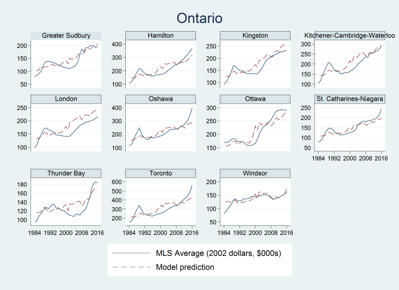 

Prices in the Prairies tend to be more closely related to the model’s predictions.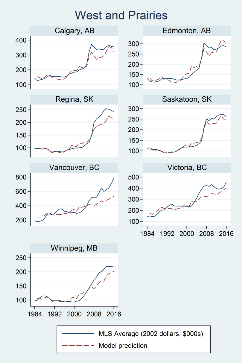

House prices in Quebec cities appear to have taken some time to catch up with (and in some cases surpass) the model’s predictions during the early 2000s, perhaps as uncertainty regarding the possibility of separation dissipated.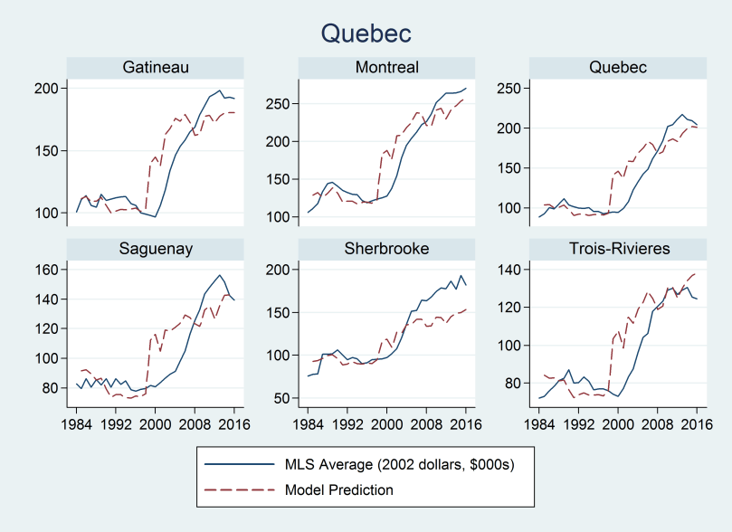

And, in the Atlantic cities, especially in St. John’s, a large increase in excess valuation of owned housing appears to be declining more recently.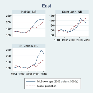

While the simplicity of the basic user-cost model makes it a tractable framework to focus on the role of interest rate expectations, it has some important limitations. Its implication that expected rent growth summarizes all of the fundamentals relevant for determining house prices is dependent on some stringent assumptions. In particular, if households’ average willingness or capacity to own rather than rent depends in a systematic way on housing quality or household incomes, both demand and supply-side factors will play a crucial role in determining the relative cost of owning and renting. For example, rising average incomes and worsening inequality in the face of geographical and regulatory constraints on land-use may result in rising average prices of owned housing relative to average rents through a composition effect: As homeowners become richer relative to renters they will buy increasingly bigger/better (and more expensive) houses.  Alternatively, if lower income households are constrained from owning as a result of credit constraints they may be forced to rent smaller and cheaper homes. 

Photo: Traditional row houses in Toronto, 2016. Photo credit: Shutterstock.